Per-channel function-node activity gating

This tutorial demonstrates node_activity_mode='per-channel' in the GSNN. We use one fixed graph and simulate two datasets from it with different special_functions per function node. Each sample carries a one-hot x_fn encoding which data-generating regime it came from (analogous to a sample-level covariate such as cell line in biology).

We compare three models on the combined dataset:

1. Model A – plain GSNN (no node-activity gating)

2. Model B – node_activity_mode='per-node' with the one-hot x_fn

3. Model C – node_activity_mode='per-channel' with the same x_fn

Per-channel gating lets a shared activity MLP produce a distinct gate for each latent channel of every function node, enabling richer condition-specific behaviour while sharing parameters across nodes.

import networkx as nx
import numpy as np
import torch
from matplotlib import pyplot as plt

from gsnn.models.GSNN import GSNN
from gsnn.simulate.nx2pyg import nx2pyg
from gsnn.simulate.simulate import simulate

%load_ext autoreload
%autoreload 2

torch.manual_seed(0)
np.random.seed(0)

device = 'cuda' if torch.cuda.is_available() else 'cpu'

Define a single graph

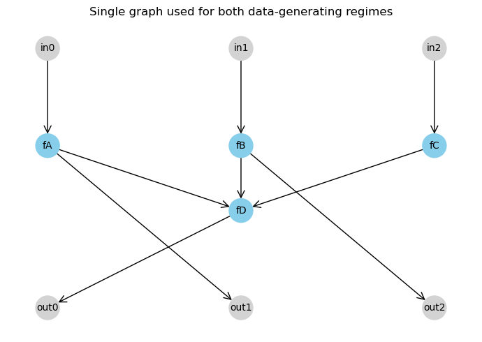
All observations share this topology. The two datasets differ only in the nonlinear functions used at each function node during simulation.

input_nodes   = ['in0', 'in1', 'in2']
function_nodes = ['fA', 'fB', 'fC', 'fD']
output_nodes  = ['out0', 'out1', 'out2']

G = nx.DiGraph()
G.add_edges_from([
    ('in0', 'fA'), ('in1', 'fB'), ('in2', 'fC'),
    ('fA', 'fD'), ('fB', 'fD'), ('fC', 'fD'),
    ('fD', 'out0'), ('fA', 'out1'), ('fB', 'out2'),
])

print(f"Graph: {G.number_of_nodes()} nodes, {G.number_of_edges()} edges")
print(f"Function nodes: {function_nodes}")

Graph: 10 nodes, 9 edges
Function nodes: ['fA', 'fB', 'fC', 'fD']

pos = {
    'in0': (-2, 2),  'in1': (0, 2),  'in2': (2, 2),
    'fA':  (-2, 0.5), 'fB': (0, 0.5), 'fC': (2, 0.5), 'fD': (0, -0.5),
    'out0': (-2, -2), 'out1': (0, -2), 'out2': (2, -2),
}

def color_for(n):
    if n in input_nodes:   return 'lightgray'
    if n in output_nodes:  return 'lightgray'
    return 'skyblue'

fig, ax = plt.subplots(figsize=(7, 5))
colors = [color_for(n) for n in G.nodes]
nx.draw_networkx(G, pos, ax=ax, node_color=colors, with_labels=True,
                 node_size=600, font_size=10, arrowstyle='->', arrowsize=18)
ax.set_title('Single graph used for both data-generating regimes')
ax.set_axis_off()
plt.tight_layout()
plt.show()

Simulate two datasets from the same graph

Each regime uses a distinct set of special_functions. We also build a one-hot condition vector per sample and broadcast it to every function node as x_fn with shape (B, Nf, 2).

special_functions_D1 = {
    'fA': lambda x: np.tanh(np.sum(x)),
    'fB': lambda x: -np.mean(x),
    'fC': lambda x: np.sum([xx**2 for xx in x]),
    'fD': lambda x: np.tanh(np.sum(x)),
}

special_functions_D2 = {
    'fA': lambda x: -np.tanh(np.sum(x)),
    'fB': lambda x: np.mean(x),
    'fC': lambda x: -np.sum([xx**2 for xx in x]),
    'fD': lambda x: -np.tanh(np.sum(x)),
}

N_TRAIN = 400
N_TEST  = 100

x_tr_1, x_te_1, y_tr_1, y_te_1 = simulate(G, n_train=N_TRAIN, n_test=N_TEST,
                                             input_nodes=input_nodes, output_nodes=output_nodes,
                                             special_functions=special_functions_D1, noise_scale=0.01)

x_tr_2, x_te_2, y_tr_2, y_te_2 = simulate(G, n_train=N_TRAIN, n_test=N_TEST,
                                             input_nodes=input_nodes, output_nodes=output_nodes,
                                             special_functions=special_functions_D2, noise_scale=0.01)

print('D1 shapes:', x_tr_1.shape, y_tr_1.shape)
print('D2 shapes:', x_tr_2.shape, y_tr_2.shape)

D1 shapes: (400, 3) (400, 3)
D2 shapes: (400, 3) (400, 3)

def condition_one_hot(n, source):
    oh = np.zeros((n, 2), dtype=np.float32)
    oh[:, source] = 1.0
    return oh

def broadcast_xfn(oh, n_fn):
    return np.broadcast_to(oh[:, None, :], (oh.shape[0], n_fn, oh.shape[1])).copy()

n_fn = len(function_nodes)

xfn_tr_1 = broadcast_xfn(condition_one_hot(N_TRAIN, 0), n_fn)
xfn_te_1 = broadcast_xfn(condition_one_hot(N_TEST,  0), n_fn)
xfn_tr_2 = broadcast_xfn(condition_one_hot(N_TRAIN, 1), n_fn)
xfn_te_2 = broadcast_xfn(condition_one_hot(N_TEST,  1), n_fn)

rng = np.random.default_rng(0)
perm = rng.permutation(2 * N_TRAIN)

def to_tensor(a):
    return torch.tensor(a, dtype=torch.float32, device=device)

x_train   = to_tensor(np.concatenate([x_tr_1, x_tr_2], axis=0)[perm])
y_train   = to_tensor(np.concatenate([y_tr_1, y_tr_2], axis=0)[perm])
xfn_train = to_tensor(np.concatenate([xfn_tr_1, xfn_tr_2], axis=0)[perm])

x_test    = to_tensor(np.concatenate([x_te_1, x_te_2], axis=0))
y_test    = to_tensor(np.concatenate([y_te_1, y_te_2], axis=0))
xfn_test  = to_tensor(np.concatenate([xfn_te_1, xfn_te_2], axis=0))

test_source = np.array(['D1'] * N_TEST + ['D2'] * N_TEST)

print('Combined train:', x_train.shape, y_train.shape, xfn_train.shape)
print('Combined test :', x_test.shape,  y_test.shape,  xfn_test.shape)
print('x_fn example (first train row, node fA):', xfn_train[0, 0].cpu().numpy())

Combined train: torch.Size([800, 3]) torch.Size([800, 3]) torch.Size([800, 4, 2])
Combined test : torch.Size([200, 3]) torch.Size([200, 3]) torch.Size([200, 4, 2])
x_fn example (first train row, node fA): [0. 1.]

Train three GSNNs on the combined dataset

• Model A sees only x and must average over both regimes.

• Model B uses per-node gating: one scalar gate per function node (identical across nodes when x_fn is broadcast).

• Model C uses per-channel gating: a vector of gates per function node from the same shared MLP.

Hyperparameters are otherwise identical.

data = nx2pyg(G, input_nodes, function_nodes, output_nodes)

gsnn_kwargs = dict(
    channels=5,
    layers=3,
    share_layers=False,
    bias=True,
    add_function_self_edges=False,
    checkpoint=False,
    norm='none',
    init='degree_normalized',
    residual=True,
    node_attn=False,
    node_mlp=False,
    dropout=0.,
)

def train(model, with_xfn, n_iters=1000, lr=1e-2, weight_decay=1e-2):
    optim = torch.optim.AdamW(model.parameters(), lr=lr, weight_decay=weight_decay)
    crit  = torch.nn.MSELoss()
    for i in range(n_iters):
        model.train(); optim.zero_grad()
        if with_xfn:
            yhat = model(x_train, x_fn=xfn_train)
        else:
            yhat = model(x_train)
        loss = crit(y_train, yhat)
        loss.backward()
        optim.step()
        if (i + 1) % 100 == 0 or i == n_iters - 1:
            model.eval()
            with torch.no_grad():
                if with_xfn:
                    yhat_te = model(x_test, x_fn=xfn_test)
                else:
                    yhat_te = model(x_test)
                te_loss = crit(y_test, yhat_te).item()
            print(f'  iter {i + 1:4d} | train mse: {loss.item():.4f} | test mse: {te_loss:.4f}', end='\r')
    print()
    return model

print('Training Model A (no node activity)...')
torch.manual_seed(0)
model_A = GSNN(data.edge_index_dict, data.node_names_dict,
               node_activity=False, **gsnn_kwargs).to(device)
train(model_A, with_xfn=False)

print('Training Model B (per-node node activity)...')
torch.manual_seed(0)
model_B = GSNN(data.edge_index_dict, data.node_names_dict,
               node_activity=True,
               node_activity_mode='per-node',
               node_activity_dim=2,
               node_activity_hidden=16,
               node_activity_temperature=0.5,
               **gsnn_kwargs).to(device)
train(model_B, with_xfn=True)

print('Training Model C (per-channel node activity)...')
torch.manual_seed(0)
model_C = GSNN(data.edge_index_dict, data.node_names_dict,
               node_activity=True,
               node_activity_mode='per-channel',
               node_activity_dim=2,
               node_activity_hidden=16,
               node_activity_temperature=0.5,
               **gsnn_kwargs).to(device)
train(model_C, with_xfn=True)

print('Model A params:', sum(p.numel() for p in model_A.parameters()))
print('Model B params:', sum(p.numel() for p in model_B.parameters()))
print('Model C params:', sum(p.numel() for p in model_C.parameters()))

Training Model A (no node activity)...
  iter 1000 | train mse: 0.4377 | test mse: 0.4625
Training Model B (per-node node activity)...
  iter 1000 | train mse: 0.2905 | test mse: 0.2792
Training Model C (per-channel node activity)...
  iter 1000 | train mse: 0.0026 | test mse: 0.0030
Model A params: 270
Model B params: 367
Model C params: 435

Test performance

model_A.eval(); model_B.eval(); model_C.eval()
with torch.no_grad():
    yhat_A = model_A(x_test).cpu().numpy()
    yhat_B = model_B(x_test, x_fn=xfn_test).cpu().numpy()
    yhat_C = model_C(x_test, x_fn=xfn_test).cpu().numpy()
y_true = y_test.cpu().numpy()

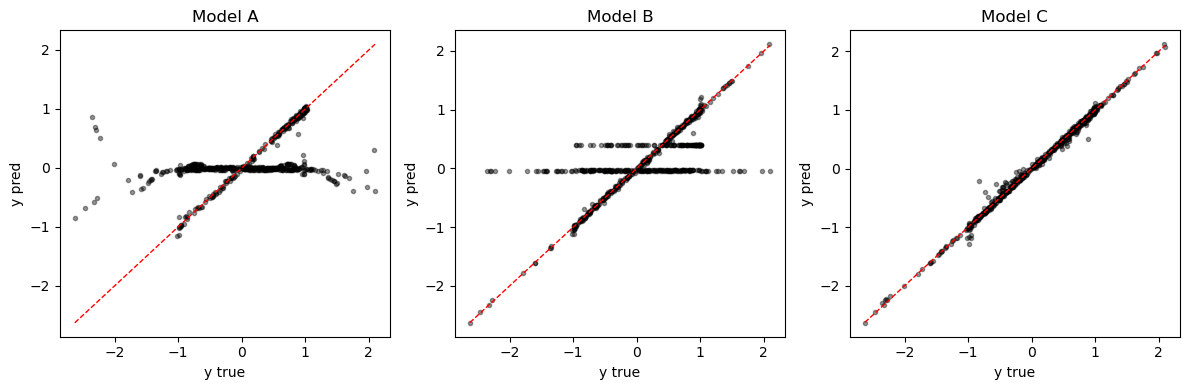
def report(name, yhat):
    mse = float(np.mean((y_true - yhat) ** 2))
    print(f'{name:>8} | test MSE: {mse:.4f}')

report('Model A', yhat_A)
report('Model B', yhat_B)
report('Model C', yhat_C)

fig, axes = plt.subplots(1, 3, figsize=(12, 4))
for ax, name, yhat in [(axes[0], 'Model A', yhat_A),
                       (axes[1], 'Model B', yhat_B),
                       (axes[2], 'Model C', yhat_C)]:
    ax.plot(y_true.ravel(), yhat.ravel(), 'k.', alpha=0.4)
    lo, hi = y_true.min(), y_true.max()
    ax.plot([lo, hi], [lo, hi], 'r--', lw=1)
    ax.set_title(name); ax.set_xlabel('y true'); ax.set_ylabel('y pred')
plt.tight_layout()
plt.show()

 Model A | test MSE: 0.4625
 Model B | test MSE: 0.2792
 Model C | test MSE: 0.0030

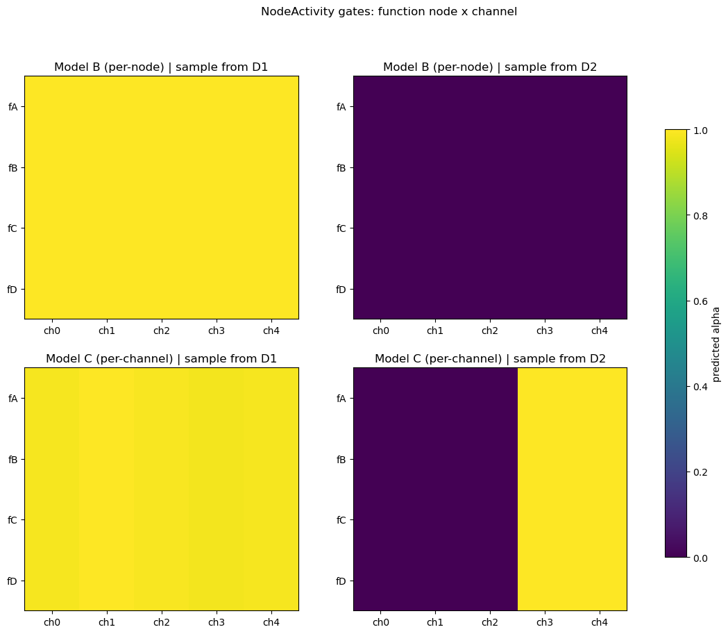
Predicted function-node activities

For Model C (per-channel), reshape the gate tensor to (Nf, C_pn) and plot heatmaps for one test sample from each regime. Under Model B (per-node), the same one-hot x_fn yields one scalar per node (constant across channels within each node).

idx_d1 = 0
idx_d2 = N_TEST

obs_d1 = x_test[idx_d1:idx_d1 + 1]
obs_d2 = x_test[idx_d2:idx_d2 + 1]
xfn_d1 = xfn_test[idx_d1:idx_d1 + 1]
xfn_d2 = xfn_test[idx_d2:idx_d2 + 1]

def gate_matrix(model, xfn_obs):
    nact = model.node_activity_model
    nact.eval()
    with torch.no_grad():
        raw = nact(xfn_obs).view(1, nact.n_nodes, nact.channels_per_node)
    return raw[0].cpu().numpy()

alpha_C_d1 = gate_matrix(model_C, xfn_d1)
alpha_C_d2 = gate_matrix(model_C, xfn_d2)
alpha_B_d1 = gate_matrix(model_B, xfn_d1)
alpha_B_d2 = gate_matrix(model_B, xfn_d2)

nact = model_C.node_activity_model
assert nact.n_nodes == len(function_nodes), (
    f"NodeActivity expects {nact.n_nodes} function nodes, notebook uses {len(function_nodes)}"
)

fig, axes = plt.subplots(2, 2, figsize=(14, 10))
panels = [
    (axes[0, 0], alpha_B_d1, 'Model B (per-node) | sample from D1'),
    (axes[0, 1], alpha_B_d2, 'Model B (per-node) | sample from D2'),
    (axes[1, 0], alpha_C_d1, 'Model C (per-channel) | sample from D1'),
    (axes[1, 1], alpha_C_d2, 'Model C (per-channel) | sample from D2'),
]
for ax, alpha, title in panels:
    im = ax.imshow(alpha, aspect='auto', vmin=0, vmax=1, cmap='viridis')
    ax.set_xticks(np.arange(alpha.shape[1]))
    ax.set_xticklabels([f'ch{c}' for c in range(alpha.shape[1])])
    ax.set_yticks(np.arange(len(function_nodes)))
    ax.set_yticklabels(function_nodes)
    ax.set_title(title)
fig.colorbar(im, ax=axes.ravel().tolist(), shrink=0.8, label='predicted alpha')
fig.suptitle('NodeActivity gates: function node x channel')
plt.show()

Takeaways

• Predictive performance: Model A must average over both data-generating regimes; Models B and C typically achieve lower test MSE because the one-hot x_fn tells the network which regime each sample came from.

• Per-node vs. per-channel: With the same one-hot x_fn broadcast to every function node, per-node mode can only apply one scalar gate per node (and the shared MLP produces the same scalar for every node given identical input). Per-channel mode learns a distinct gate for each latent channel, enabling richer condition-specific modulation with parameter sharing across nodes.

• Extensions: Replace the one-hot with real sample-level covariates (e.g. cell-line embeddings), increase node_activity_dim, or add more regimes — the same per-channel machinery applies.