Function-node activity gating

This tutorial demonstrates the node_activity feature of the GSNN. We simulate data from two overlapping graphs (shared inputs/outputs, but different function nodes). A single GSNN is trained on the union graph and receives a per-sample binary vector x_fn telling it which function nodes are active for that sample.

We compare two models:

1. Model A – plain GSNN (no node-activity gating)

2. Model B – GSNN with node_activity=True, conditioned on the binary x_fn

We then use GSNNExplainer to extract per-observation node importances and check, for one observation from each graph, whether the explainer’s top-ranked function nodes align with the true set of function nodes used to generate that observation.

import networkx as nx
import numpy as np
import torch
from matplotlib import pyplot as plt
from sklearn.metrics import roc_auc_score

from gsnn.models.GSNN import GSNN
from gsnn.simulate.nx2pyg import nx2pyg
from gsnn.simulate.simulate import simulate
from gsnn.interpret import GSNNExplainer

%load_ext autoreload
%autoreload 2

torch.manual_seed(0)
np.random.seed(0)

device = 'cuda' if torch.cuda.is_available() else 'cpu'

Define two overlapping graphs

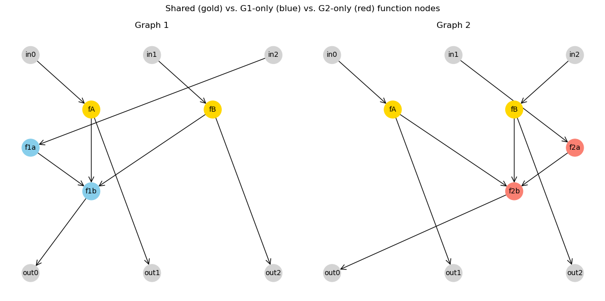
Both graphs share the same input nodes (in0..in2), output nodes (out0..out2), and two shared function nodes (fA, fB). Each graph adds a pair of unique function nodes that route information differently.

The GSNN is constructed on the union of the two graphs so a single model architecture can represent both data-generating processes.

input_nodes  = ['in0', 'in1', 'in2']
output_nodes = ['out0', 'out1', 'out2']

shared_fns = ['fA', 'fB']
only_G1    = ['f1a', 'f1b']
only_G2    = ['f2a', 'f2b']
function_nodes = shared_fns + only_G1 + only_G2  # union ordering

# Graph 1: routes through fA/fB and the f1* nodes
G1 = nx.DiGraph()
G1.add_edges_from([
    ('in0', 'fA'),  ('in1', 'fB'),  ('in2', 'f1a'),
    ('fA',  'f1b'), ('fB',  'f1b'), ('f1a', 'f1b'),
    ('f1b', 'out0'), ('fA', 'out1'), ('fB', 'out2'),
])

# Graph 2: routes through fA/fB and the f2* nodes
G2 = nx.DiGraph()
G2.add_edges_from([
    ('in0', 'fA'),  ('in1', 'f2a'), ('in2', 'fB'),
    ('fA',  'f2b'), ('fB',  'f2b'), ('f2a', 'f2b'),
    ('f2b', 'out0'), ('fA', 'out1'), ('fB', 'out2'),
])

# Union graph used to build the GSNN (also ensures every node/edge appears)
G_union = nx.compose(G1, G2)
for n in input_nodes + function_nodes + output_nodes:
    G_union.add_node(n)

print(f"G1: {G1.number_of_nodes()} nodes, {G1.number_of_edges()} edges")
print(f"G2: {G2.number_of_nodes()} nodes, {G2.number_of_edges()} edges")
print(f"Union: {G_union.number_of_nodes()} nodes, {G_union.number_of_edges()} edges")
print(f"Function-node ordering: {function_nodes}")

G1: 10 nodes, 9 edges
G2: 10 nodes, 9 edges
Union: 12 nodes, 15 edges
Function-node ordering: ['fA', 'fB', 'f1a', 'f1b', 'f2a', 'f2b']

# Side-by-side plot of the two source graphs
pos = {
    'in0': (-2, 2),  'in1': (0, 2),  'in2': (2, 2),
    'fA':  (-1, 1),  'fB':  (1, 1),
    'f1a': (-2, 0.3),'f1b': (-1, -0.5),
    'f2a': (2, 0.3), 'f2b': (1, -0.5),
    'out0': (-2, -2),'out1': (0, -2), 'out2': (2, -2),
}

def color_for(n):
    if n in input_nodes:   return 'lightgray'
    if n in output_nodes:  return 'lightgray'
    if n in shared_fns:    return 'gold'
    if n in only_G1:       return 'skyblue'
    if n in only_G2:       return 'salmon'
    return 'white'

fig, axes = plt.subplots(1, 2, figsize=(12, 6))
for ax, G, title in [(axes[0], G1, 'Graph 1'), (axes[1], G2, 'Graph 2')]:
    sub_pos = {n: pos[n] for n in G.nodes}
    colors = [color_for(n) for n in G.nodes]
    nx.draw_networkx(G, sub_pos, ax=ax, node_color=colors, with_labels=True,
                     node_size=600, font_size=10, arrowstyle='->', arrowsize=18)
    ax.set_title(title)
    ax.set_axis_off()
plt.suptitle('Shared (gold) vs. G1-only (blue) vs. G2-only (red) function nodes')
plt.tight_layout()
plt.show()

Simulate data from each graph

We use the standard Bayesian-network simulator. A small set of per-graph special_functions ensures the two data-generating processes behave differently. For every sample we also record a length-|function_nodes| binary mask indicating which function nodes belong to the source graph (this is the x_fn input the node-activity model will use).

special_functions_G1 = {
    'fA':  lambda x: np.tanh(np.sum(x)),
    'fB':  lambda x: -np.mean(x),
    'f1a': lambda x: np.sum([xx**2 for xx in x]),
    'f1b': lambda x: np.tanh(np.sum(x)),
}

special_functions_G2 = {
    'fA':  lambda x: np.tanh(np.sum(x)),
    'fB':  lambda x: -np.mean(x),
    'f2a': lambda x: -np.sum([xx**2 for xx in x]),
    'f2b': lambda x: -np.tanh(np.sum(x)),
}

N_TRAIN = 400
N_TEST  = 100

x_tr_1, x_te_1, y_tr_1, y_te_1 = simulate(G1, n_train=N_TRAIN, n_test=N_TEST,
                                           input_nodes=input_nodes, output_nodes=output_nodes,
                                           special_functions=special_functions_G1, noise_scale=0.01)

x_tr_2, x_te_2, y_tr_2, y_te_2 = simulate(G2, n_train=N_TRAIN, n_test=N_TEST,
                                           input_nodes=input_nodes, output_nodes=output_nodes,
                                           special_functions=special_functions_G2, noise_scale=0.01)

print('G1 shapes:', x_tr_1.shape, y_tr_1.shape)
print('G2 shapes:', x_tr_2.shape, y_tr_2.shape)

G1 shapes: (400, 3) (400, 3)
G2 shapes: (400, 3) (400, 3)

# Per-graph function-node activity masks (1 = node present in that graph's subgraph)
def activity_vector(G_sub, function_nodes):
    present = set(G_sub.nodes)
    return np.array([1.0 if n in present else 0.0 for n in function_nodes], dtype=np.float32)

fn_mask_G1 = activity_vector(G1, function_nodes)
fn_mask_G2 = activity_vector(G2, function_nodes)

print('fn_mask_G1:', dict(zip(function_nodes, fn_mask_G1.astype(int))))
print('fn_mask_G2:', dict(zip(function_nodes, fn_mask_G2.astype(int))))

# Broadcast per-graph masks to per-sample masks
xfn_tr_1 = np.broadcast_to(fn_mask_G1, (N_TRAIN, len(function_nodes))).copy()
xfn_te_1 = np.broadcast_to(fn_mask_G1, (N_TEST,  len(function_nodes))).copy()
xfn_tr_2 = np.broadcast_to(fn_mask_G2, (N_TRAIN, len(function_nodes))).copy()
xfn_te_2 = np.broadcast_to(fn_mask_G2, (N_TEST,  len(function_nodes))).copy()

# Combine into one shuffled train set and one stacked test set (graph 1 first, then graph 2)
rng = np.random.default_rng(0)
perm = rng.permutation(2 * N_TRAIN)

def to_tensor(a):
    return torch.tensor(a, dtype=torch.float32, device=device)

x_train   = to_tensor(np.concatenate([x_tr_1, x_tr_2], axis=0)[perm])
y_train   = to_tensor(np.concatenate([y_tr_1, y_tr_2], axis=0)[perm])
xfn_train = to_tensor(np.concatenate([xfn_tr_1, xfn_tr_2], axis=0)[perm])

x_test    = to_tensor(np.concatenate([x_te_1, x_te_2], axis=0))
y_test    = to_tensor(np.concatenate([y_te_1, y_te_2], axis=0))
xfn_test  = to_tensor(np.concatenate([xfn_te_1, xfn_te_2], axis=0))

# Track which source graph each test row came from (for later evaluation)
test_source = np.array(['G1'] * N_TEST + ['G2'] * N_TEST)

print('Combined train:', x_train.shape, y_train.shape, xfn_train.shape)
print('Combined test :', x_test.shape,  y_test.shape,  xfn_test.shape)

fn_mask_G1: {'fA': 1, 'fB': 1, 'f1a': 1, 'f1b': 1, 'f2a': 0, 'f2b': 0}
fn_mask_G2: {'fA': 1, 'fB': 1, 'f1a': 0, 'f1b': 0, 'f2a': 1, 'f2b': 1}
Combined train: torch.Size([800, 3]) torch.Size([800, 3]) torch.Size([800, 6])
Combined test : torch.Size([200, 3]) torch.Size([200, 3]) torch.Size([200, 6])

Train two GSNNs on the combined dataset

• Model A sees only x. It cannot distinguish which source graph a sample came from, so it has to learn an average behaviour over both.

• Model B sees x and the binary x_fn mask. The NodeActivity module produces a per-function-node gate (one scalar per node, shared across all layers).

Hyperparameters are otherwise identical.

data = nx2pyg(G_union, input_nodes, function_nodes, output_nodes)

gsnn_kwargs = dict(
    channels=5,
    layers=3,
    share_layers=False,
    bias=True,
    add_function_self_edges=False,
    checkpoint=False,
    norm='none',
    init='degree_normalized',
    residual=True,
    node_attn=False,
    node_mlp=False,
    dropout=0.,
)

def train(model, with_xfn, n_iters=1000, lr=1e-2, weight_decay=1e-2):
    optim = torch.optim.AdamW(model.parameters(), lr=lr, weight_decay=weight_decay)
    crit  = torch.nn.MSELoss()
    for i in range(n_iters):
        model.train(); optim.zero_grad()
        if with_xfn:
            yhat = model(x_train, x_fn=xfn_train)
        else:
            yhat = model(x_train)
        loss = crit(y_train, yhat)
        loss.backward()
        optim.step()
        if (i + 1) % 100 == 0 or i == n_iters - 1:
            model.eval()
            with torch.no_grad():
                if with_xfn:
                    yhat_te = model(x_test, x_fn=xfn_test)
                else:
                    yhat_te = model(x_test)
                te_loss = crit(y_test, yhat_te).item()
            print(f'  iter {i + 1:4d} | train mse: {loss.item():.4f} | test mse: {te_loss:.4f}', end='\r')
    print()
    return model

print('Training Model A (no node activity)...')
torch.manual_seed(0)
model_A = GSNN(data.edge_index_dict, data.node_names_dict,
               node_activity=False, **gsnn_kwargs).to(device)
train(model_A, with_xfn=False)

print('Training Model B (with node activity)...')
torch.manual_seed(0)
model_B = GSNN(data.edge_index_dict, data.node_names_dict,
               node_activity=True,
               node_activity_dim=1,
               node_activity_hidden=16,
               node_activity_temperature=0.5,
               **gsnn_kwargs).to(device)
train(model_B, with_xfn=True)

print('Model A params:', sum(p.numel() for p in model_A.parameters()))
print('Model B params:', sum(p.numel() for p in model_B.parameters()))

Training Model A (no node activity)...
  iter 1000 | train mse: 0.2516 | test mse: 0.2494
Training Model B (with node activity)...
  iter 1000 | train mse: 0.1590 | test mse: 0.1566
Model A params: 453
Model B params: 534

Test performance

model_A.eval(); model_B.eval()
with torch.no_grad():
    yhat_A = model_A(x_test).cpu().numpy()
    yhat_B = model_B(x_test, x_fn=xfn_test).cpu().numpy()
y_true = y_test.cpu().numpy()

def report(name, yhat):
    mse = float(np.mean((y_true - yhat) ** 2))
    r   = float(np.corrcoef(y_true.ravel(), yhat.ravel())[0, 1])
    print(f'{name}: test MSE = {mse:.4f} | Pearson r = {r:.4f}')

report('Model A (no node activity)', yhat_A)
report('Model B (with node activity)', yhat_B)

fig, axes = plt.subplots(1, 2, figsize=(10, 5), sharex=True, sharey=True)
for ax, name, yhat in [(axes[0], 'Model A', yhat_A), (axes[1], 'Model B', yhat_B)]:
    ax.plot(y_true.ravel(), yhat.ravel(), 'k.', alpha=0.4)
    lo, hi = y_true.min(), y_true.max()
    ax.plot([lo, hi], [lo, hi], 'r--', lw=1)
    ax.set_title(name); ax.set_xlabel('y true'); ax.set_ylabel('y pred')
plt.tight_layout()
plt.show()

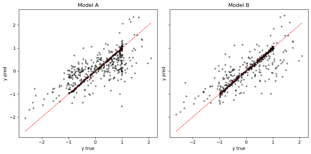
Model A (no node activity): test MSE = 0.2494 | Pearson r = 0.7756
Model B (with node activity): test MSE = 0.1566 | Pearson r = 0.8659

Per-observation node importances

We pick one test observation from each source graph and run GSNNExplainer to extract per-node importance scores. For Model B we forward x_fn to the underlying GSNN through the explainer’s new model_kwargs hook.

Ground truth: for an observation drawn from graph G_i, the true set of “important” function nodes is the set of function nodes that appear in G_i and lie on some input→output path. Function nodes that are only in the other graph should receive low scores.

# Pick one observation from each source graph
idx_1 = 0                     # first row in test set came from G1
idx_2 = N_TEST                # first row from G2

obs_1     = x_test[idx_1:idx_1 + 1]
obs_2     = x_test[idx_2:idx_2 + 1]
xfn_obs_1 = xfn_test[idx_1:idx_1 + 1]
xfn_obs_2 = xfn_test[idx_2:idx_2 + 1]

# Ground-truth active function nodes per graph: those reachable on an input->output path
def active_function_nodes(G_sub, input_nodes, output_nodes, function_nodes):
    reachable_from_inputs = set()
    for s in input_nodes:
        if s in G_sub:
            reachable_from_inputs |= nx.descendants(G_sub, s)
    can_reach_outputs = set()
    for t in output_nodes:
        if t in G_sub:
            can_reach_outputs |= nx.ancestors(G_sub, t)
    active = reachable_from_inputs & can_reach_outputs
    return [n for n in function_nodes if n in active]

active_G1 = active_function_nodes(G1, input_nodes, output_nodes, function_nodes)
active_G2 = active_function_nodes(G2, input_nodes, output_nodes, function_nodes)

print('Active function nodes in G1:', active_G1)
print('Active function nodes in G2:', active_G2)

Active function nodes in G1: ['fA', 'fB', 'f1a', 'f1b']
Active function nodes in G2: ['fA', 'fB', 'f2a', 'f2b']

EXPLAINER_KWARGS = dict(iters=300, beta=1e-2, lr=1e-2, prior=1.0, verbose=True)

def explain_node(model, obs, model_kwargs=None):
    expl = GSNNExplainer(model, data, **EXPLAINER_KWARGS)
    return expl.explain(obs, target='node', model_kwargs=model_kwargs)

node_df_A_1 = explain_node(model_A, obs_1)
node_df_A_2 = explain_node(model_A, obs_2)
node_df_B_1 = explain_node(model_B, obs_1, model_kwargs={'x_fn': xfn_obs_1})
node_df_B_2 = explain_node(model_B, obs_2, model_kwargs={'x_fn': xfn_obs_2})

print('Top-5 nodes per (model, observation):')
for name, df in [('A | obs from G1', node_df_A_1), ('A | obs from G2', node_df_A_2),
                 ('B | obs from G1', node_df_B_1), ('B | obs from G2', node_df_B_2)]:
    top = df.sort_values('score', ascending=False).head(5)
    print(f'  {name:>20}: ' + ', '.join(f'{n}={s:.2f}' for n, s in zip(top['node'], top['score'])))

iter: 299 | loss: 0.1118 | mse: 0.0447 | r2: 0.933 | active nodes: 7 / 12 | entropy: 0.21276
==================================================
POST-TRAINING EVALUATION (nodes > 0.5)
==================================================
Selected nodes: 6 / 12 (50.0%)
MSE (subset): 0.000000
R² (subset): 1.0000
==================================================
iter: 299 | loss: 0.0545 | mse: 0.0045 | r2: 0.993 | active nodes: 5 / 12 | entropy: 0.2081
==================================================
POST-TRAINING EVALUATION (nodes > 0.5)
==================================================
Selected nodes: 4 / 12 (33.3%)
MSE (subset): 0.061055
R² (subset): 0.9664
==================================================
iter: 299 | loss: 0.0430 | mse: 0.0001 | r2: 1.000 | active nodes: 5 / 12 | entropy: 0.18669
==================================================
POST-TRAINING EVALUATION (nodes > 0.5)
==================================================
Selected nodes: 3 / 12 (25.0%)
MSE (subset): 0.000103
R² (subset): 0.9998
==================================================
iter: 299 | loss: 0.0401 | mse: 0.0000 | r2: 1.000 | active nodes: 4 / 12 | entropy: 0.12375
==================================================
POST-TRAINING EVALUATION (nodes > 0.5)
==================================================
Selected nodes: 4 / 12 (33.3%)
MSE (subset): 0.000000
R² (subset): 1.0000
==================================================
Top-5 nodes per (model, observation):
       A | obs from G1: fA=0.99, f1b=0.97, f2b=0.96, f1a=0.92, fB=0.85
       A | obs from G2: fA=0.99, fB=0.99, f2a=0.90, f2b=0.88, f1b=0.27
       B | obs from G1: fA=0.99, f1b=0.99, fB=0.89, f1a=0.44, f2b=0.04
       B | obs from G2: fA=0.99, fB=0.99, f2a=0.98, f2b=0.97, f1a=0.04

# Quantitative comparison: restrict to function nodes (inputs/outputs are not part of the ground truth)
def fn_scores(df):
    sub = df[df['node'].isin(function_nodes)].set_index('node').reindex(function_nodes)
    return sub['score'].to_numpy()

def precision_at_k(scores, truth_mask, k):
    order = np.argsort(-scores)
    return float(truth_mask[order[:k]].mean())

def auroc(scores, truth_mask):
    if truth_mask.sum() in (0, len(truth_mask)):
        return float('nan')
    return float(roc_auc_score(truth_mask, scores))

def evaluate(df, active_set):
    scores = fn_scores(df)
    truth  = np.array([1 if n in active_set else 0 for n in function_nodes], dtype=int)
    k      = int(truth.sum())
    return {
        'precision@k': precision_at_k(scores, truth, k),
        'AUROC':       auroc(scores, truth),
        'k':           k,
    }

rows = []
for label, df, active in [
    ('A | obs from G1', node_df_A_1, active_G1),
    ('A | obs from G2', node_df_A_2, active_G2),
    ('B | obs from G1', node_df_B_1, active_G1),
    ('B | obs from G2', node_df_B_2, active_G2),
]:
    m = evaluate(df, active)
    rows.append((label, m['k'], m['precision@k'], m['AUROC']))

print(f'{"setting":>20} | {"k":>2} | {"prec@k":>7} | {"AUROC":>6}')
print('-' * 48)
for label, k, p, a in rows:
    print(f'{label:>20} | {k:>2d} | {p:>7.3f} | {a:>6.3f}')

             setting |  k |  prec@k |  AUROC
------------------------------------------------
     A | obs from G1 |  4 |   0.750 |  0.750
     A | obs from G2 |  4 |   1.000 |  1.000
     B | obs from G1 |  4 |   1.000 |  1.000
     B | obs from G2 |  4 |   1.000 |  1.000

# Bar plot: per-function-node scores, colored by ground truth membership in the source graph
fig, axes = plt.subplots(2, 2, figsize=(12, 7), sharey=True)
panels = [
    (axes[0, 0], node_df_A_1, active_G1, 'Model A | obs from G1'),
    (axes[0, 1], node_df_A_2, active_G2, 'Model A | obs from G2'),
    (axes[1, 0], node_df_B_1, active_G1, 'Model B | obs from G1'),
    (axes[1, 1], node_df_B_2, active_G2, 'Model B | obs from G2'),
]
for ax, df, active, title in panels:
    scores = fn_scores(df)
    colors = ['tab:green' if n in active else 'tab:red' for n in function_nodes]
    ax.bar(function_nodes, scores, color=colors)
    ax.set_title(title)
    ax.set_ylim(0, 1)
    ax.tick_params(axis='x', rotation=45)
axes[0, 0].set_ylabel('score')
axes[1, 0].set_ylabel('score')
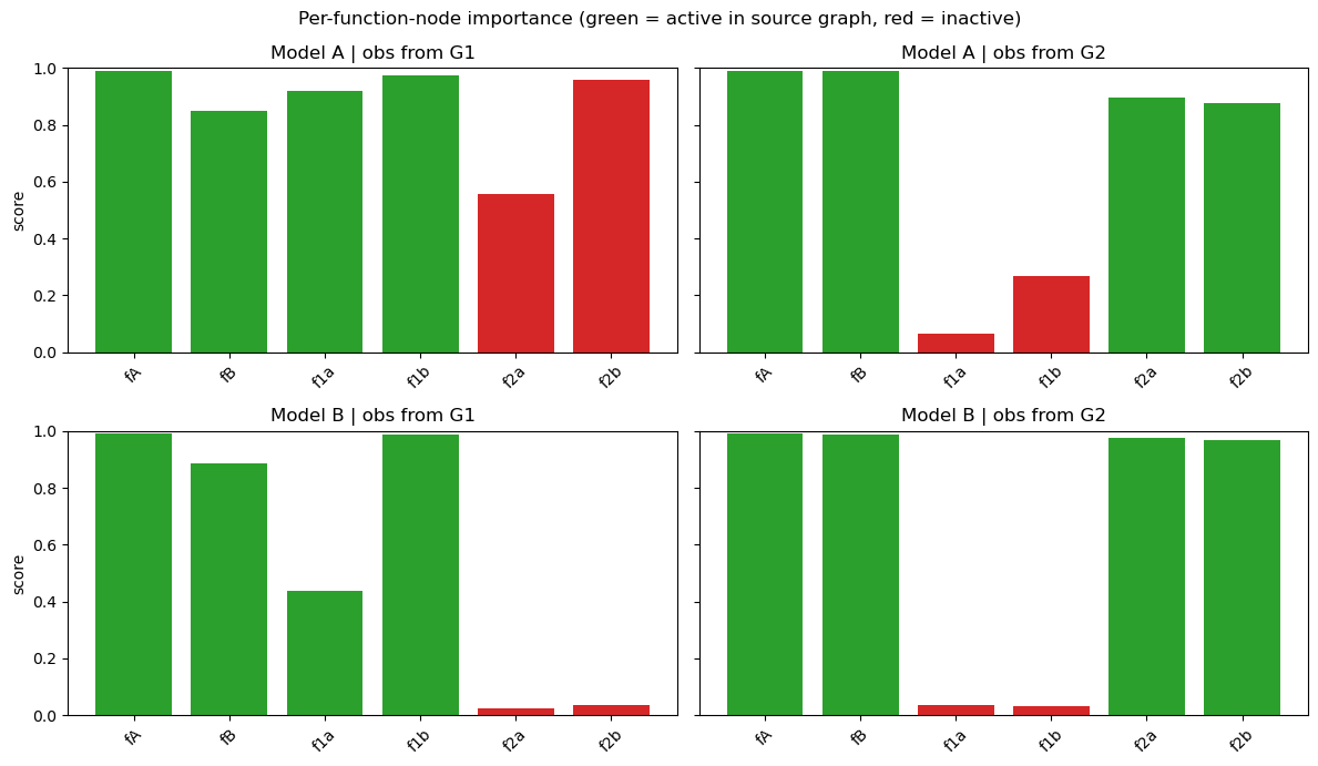
fig.suptitle('Per-function-node importance (green = active in source graph, red = inactive)')
plt.tight_layout()
plt.show()

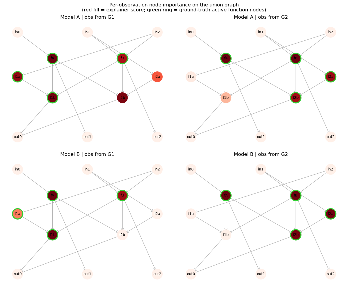
# Same four explanations rendered on the union-graph topology.
# Node fill = explainer score (red shade), green outline = ground-truth active in source graph.
fig, axes = plt.subplots(2, 2, figsize=(12, 10))
panels = [
    (axes[0, 0], node_df_A_1, 'Model A | obs from G1', active_G1),
    (axes[0, 1], node_df_A_2, 'Model A | obs from G2', active_G2),
    (axes[1, 0], node_df_B_1, 'Model B | obs from G1', active_G1),
    (axes[1, 1], node_df_B_2, 'Model B | obs from G2', active_G2),
]
for ax, df, title, active in panels:
    score_map = dict(zip(df['node'], df['score']))
    node_colors = [score_map.get(n, 0.0) for n in G_union.nodes]
    nx.draw_networkx_edges(G_union, pos, ax=ax, arrowstyle='->', arrowsize=15,
                           edge_color='gray', alpha=0.6)
    nx.draw_networkx_labels(G_union, pos, ax=ax, font_size=9)
    nx.draw_networkx_nodes(G_union, pos, ax=ax, nodelist=list(G_union.nodes),
                           node_color=node_colors, cmap=plt.cm.Reds,
                           vmin=0, vmax=1, node_size=650)
    active_in_graph = [n for n in active if n in G_union.nodes]
    if active_in_graph:
        nx.draw_networkx_nodes(G_union, pos, ax=ax, nodelist=active_in_graph,
                               node_color='none', edgecolors='limegreen',
                               linewidths=2.5, node_size=650)
    ax.set_title(title)
    ax.set_axis_off()
plt.suptitle('Per-observation node importance on the union graph\n'
             '(red fill = explainer score; green ring = ground-truth active function nodes)')
plt.tight_layout()
plt.show()

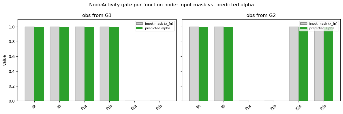
Predicted function-node activities (Model B)

We can also inspect the gates that NodeActivity produces directly. For each sample the module runs the binary x_fn through a small MLP and a sigmoid to yield one scalar alpha per function node, which is then broadcast across that node’s channels at every layer.

A well-trained gate should output alpha ≈ 1 for function nodes that are active in the source graph and alpha ≈ 0 for the ones that are not. Below we plot the predicted alpha next to the input mask for one observation from each graph.

# Extract per-function-node alpha from NodeActivity.
# NodeActivity returns (B, Nf*C_pn) by broadcasting alpha across each node's channels,
# so the per-node gate is recovered by reshaping and taking any channel slot.
nact = model_B.node_activity_model
nact.eval()
with torch.no_grad():
    raw_1 = nact(xfn_obs_1).view(1, nact.n_nodes, nact.channels_per_node)
    raw_2 = nact(xfn_obs_2).view(1, nact.n_nodes, nact.channels_per_node)
    alpha_1 = raw_1[0, :, 0].cpu().numpy()
    alpha_2 = raw_2[0, :, 0].cpu().numpy()

assert nact.n_nodes == len(function_nodes), (
    f"NodeActivity expects {nact.n_nodes} function nodes, notebook uses {len(function_nodes)}"
)

fig, axes = plt.subplots(1, 2, figsize=(12, 4), sharey=True)
panels = [
    (axes[0], alpha_1, xfn_obs_1[0].cpu().numpy(), 'obs from G1', active_G1),
    (axes[1], alpha_2, xfn_obs_2[0].cpu().numpy(), 'obs from G2', active_G2),
]
xpos = np.arange(len(function_nodes))
width = 0.38
for ax, alpha, mask, title, active in panels:
    bar_colors = ['tab:green' if n in active else 'tab:red' for n in function_nodes]
    ax.bar(xpos - width / 2, mask, width=width, color='lightgray',
           edgecolor='gray', label='input mask (x_fn)')
    ax.bar(xpos + width / 2, alpha, width=width, color=bar_colors,
           label='predicted alpha')
    ax.axhline(0.5, color='k', lw=0.5, ls=':')
    ax.set_xticks(xpos)
    ax.set_xticklabels(function_nodes, rotation=45)
    ax.set_ylim(0, 1.1)
    ax.set_title(title)
    ax.legend(loc='upper right', fontsize=8)
axes[0].set_ylabel('value')
fig.suptitle('NodeActivity gate per function node: input mask vs. predicted alpha')
plt.tight_layout()
plt.show()

Takeaways

• Predictive performance: Model B (with node_activity) typically achieves lower test MSE because the binary x_fn mask lets a single GSNN cleanly separate the two data-generating processes; Model A has to average over both.

• Node importances: Because Model B’s NodeActivity gates suppress channels of function nodes that are not active in a given sample, the explainer is forced to attribute predictions only to the active subset. Model A has no such mechanism, so its node importances tend to spread across function nodes from both source graphs, lowering precision@k and AUROC against the ground-truth active set.

This is the simplest possible demonstration — the same setup can be extended to richer per-node features (node_activity_dim > 1), more than two graphs, or more realistic biology-inspired pathways.