[1]:
import networkx as nx
from matplotlib import pyplot as plt
import numpy as np
import networkx as nx
import torch

from gsnn.models.GSNN import GSNN
from gsnn.simulate.nx2pyg import nx2pyg
from gsnn.simulate.datasets import simulate_3_in_3_out
from gsnn.interpret.GSNNExplainer import GSNNExplainer
from gsnn.interpret.IGExplainer import IGExplainer
from gsnn.interpret.ContrastiveIGExplainer import ContrastiveIGExplainer
from gsnn.interpret.NoiseTunnel import NoiseTunnel
from gsnn.interpret.ContrastiveOcclusionExplainer import ContrastiveOcclusionExplainer
from gsnn.interpret.OcclusionExplainer import OcclusionExplainer
from gsnn.interpret.utils import plot_edge_importance, plot_node_importance
from gsnn.interpret.CounterfactualExplainer import CounterfactualExplainer

# for reproducibility
torch.manual_seed(0)
np.random.seed(0)

%load_ext autoreload
%autoreload 2
/home/teddy/miniconda3/envs/gsnn-mds/lib/python3.12/site-packages/tqdm/auto.py:21: TqdmWarning: IProgress not found. Please update jupyter and ipywidgets. See https://ipywidgets.readthedocs.io/en/stable/user_install.html
  from .autonotebook import tqdm as notebook_tqdm
GSNN Interpretation methods
[2]:
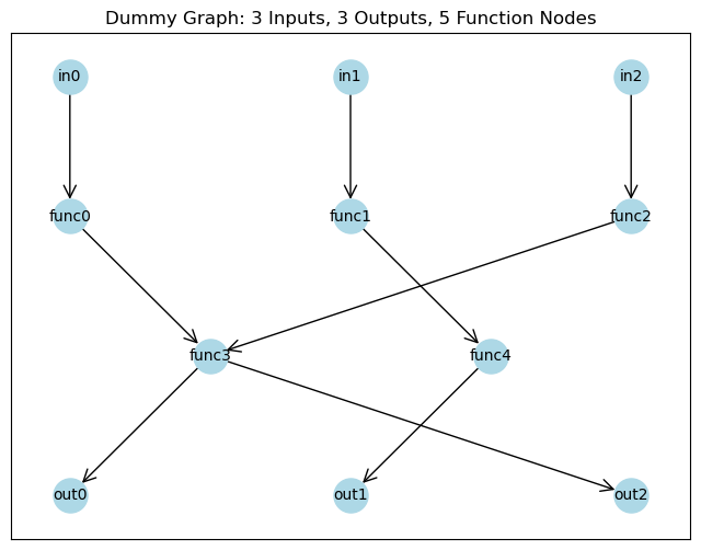
G, pos, x_train, x_test, y_train, y_test, \
    input_nodes, function_nodes, output_nodes = simulate_3_in_3_out(n_train=500,
                                                                    n_test=100,
                                                                    noise_scale=0.1,
                                                                    device='cuda')

plt.figure(figsize=(8, 6))
nx.draw_networkx(G, pos, with_labels=True, node_color='lightblue', node_size=500, font_size=10, arrowstyle='->', arrowsize=20)
plt.title("Dummy Graph: 3 Inputs, 3 Outputs, 5 Function Nodes")
plt.show()
[3]:
device = torch.device('cuda' if torch.cuda.is_available() else 'cpu')

data = nx2pyg(G, input_nodes, function_nodes, output_nodes)

model = GSNN(data.edge_index_dict,
             data.node_names_dict,
             channels=20,
             layers=2,
             dropout=0.1,
             share_layers=True,
             bias=False,
             add_function_self_edges=False,
             checkpoint=False,
             norm='batch',
             residual=True).to(device)

print('n params', sum([p.numel() for p in model.parameters()]))

optim = torch.optim.AdamW(model.parameters(), lr=1e-2, weight_decay=1e-2)
crit = torch.nn.MSELoss()

for i in range(1000):
    model.train()
    optim.zero_grad()

    yhat = model(x_train)
    loss = crit(y_train, yhat)
    loss.backward()
    optim.step()

    model.eval()
    with torch.no_grad():
        yhat = model(x_test)
        loss = crit(y_test, yhat)

    print(f'iter: {i} | loss: {loss.item():.3f}',end='\r')

model = model.eval()
n params 11218
iter: 999 | loss: 0.225
Explanations of multiple observations with GSNNExplainer
The GSNN explainer method is inspired by GNNExplainer proposed by Ying et. al., however, our approaches diverges slightly in a number of ways:
We use MSE rather than mutual information as the optimization objective
We use gumbel-softmax to discretize edge weights [0,1]
We focus on edge explanations rather than node or feature explanations
@misc{ying2019gnnexplainergeneratingexplanationsgraph,
      title={GNNExplainer: Generating Explanations for Graph Neural Networks},
      author={Rex Ying and Dylan Bourgeois and Jiaxuan You and Marinka Zitnik and Jure Leskovec},
      year={2019},
      eprint={1903.03894},
      archivePrefix={arXiv},
      primaryClass={cs.LG},
      url={https://arxiv.org/abs/1903.03894},
}
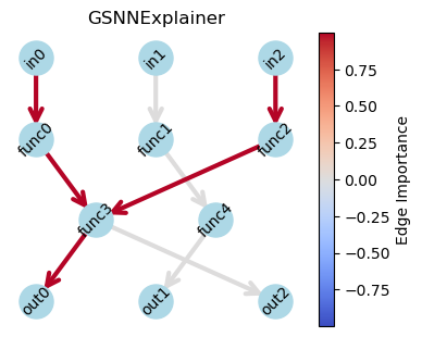
GSNNExplainer attempts to identify a minimal subgraph that can faithfully reproduce equivalent predictions. This explanation can be used with multiple samples and targets. The resulting edge scores indicate the probability of inclusion:
NOTE: it is important to tune the parameters to ensure faithful predictions. Using too strong of regularization (large beta) can result in unfaithful predictions. We have included a tune function to adjust beta to a maximum value while maintaining an explained variance threshold (default: 0.7).
[4]:
target_ixs = [0]

explainer = GSNNExplainer(model, data, ignore_cuda=False, gumbel_softmax=True, hard=False, tau0=10, min_tau=0.5,
                            prior=2, iters=500, lr=1e-2, weight_decay=0, beta=1, verbose=True,
                            optimizer=torch.optim.Adam, free_edges=0)

# res = explainer.explain(x_train, targets=target_ixs)
tune_dict = explainer.tune(x_train, targets=target_ixs, min_r2=0.7)
res = tune_dict['edge_df']

plot_edge_importance(res, pos, title='GSNNExplainer')
============================================================
BETA TUNING - Starting from User's Beta
============================================================
Target: Find max beta with R² >= 0.700
Starting beta: 1.0000
Step size: 1.50x
============================================================

Step 1: Evaluating starting beta = 1.0000
  → R² = -0.0321, Edges = 2
  ✗ Poor performance! Searching downward for better performance...

Trial 1: Testing beta = 0.6667 (direction: down)
  → R² = 0.5909, Edges = 4
  ✗ Still poor, continuing downward...

Trial 2: Testing beta = 0.4444 (direction: down)
  → R² = 1.0000, Edges = 5
  ✓ Performance recovered! Optimal: β=0.4444

============================================================
TUNING COMPLETE
============================================================
Starting beta: 1.0000
Optimal beta: 0.4444
Change: 0.44x
Final R²: 1.0000
Selected edges: 5 / 9 (55.6%)
============================================================
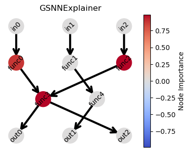
Optionally choose node or edge attribution
[15]:
target_ixs = [0]

explainer = GSNNExplainer(model, data, ignore_cuda=False, gumbel_softmax=True, hard=False, tau0=10, min_tau=0.5,
                            prior=2, iters=500, lr=1e-2, weight_decay=0, beta=1, verbose=True,
                            optimizer=torch.optim.Adam, free_edges=0)

res = explainer.explain(x_train, targets=target_ixs, target='node')

plot_node_importance(res, G, pos, title='GSNNExplainer')
iter: 499 | loss: 2.9578 | mse: 0.0019 | r2: 0.999 | active nodes: 3 / 11 | entropy: 0.06778
==================================================
POST-TRAINING EVALUATION (nodes > 0.5)
==================================================
Selected nodes: 3 / 11 (27.3%)
MSE (subset): 0.000000
R² (subset): 1.0000
Variance explained: 1.0000
Correlation: 1.0000
==================================================
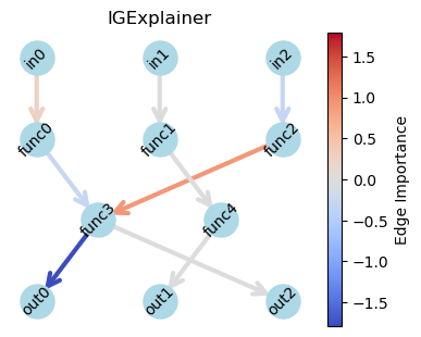
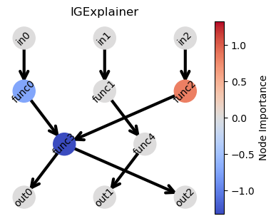
Explanations of a single observation with Integrated Gradients
“What latent edge features are responsible for an observations predicted outcome?”
In some cases, injecting noise can help provide more robust explanations. More information here. In this example, it is comparable to contrastive_ig.
[6]:
x = x_train[[0]]
y = y_train[[0]]
target_ixs = [0]

explainer = NoiseTunnel(IGExplainer(model, data), n_samples=100, noise_std=0.1, agg='mean')

res = explainer.explain(x, target_idx=target_ixs)
res = res.sort_values('score', ascending=False)

plot_edge_importance(res, pos, title='IGExplainer')
res.sort_values('score', ascending=False)
[6]:
| source | target | score | |
|---|---|---|---|
| 2 | func2 | func3 | 0.911708 |
| 3 | in0 | func0 | 0.263096 |
| 8 | func4 | out1 | 0.000000 |
| 1 | func1 | func4 | 0.000000 |
| 4 | in1 | func1 | 0.000000 |
| 7 | func3 | out2 | 0.000000 |
| 0 | func0 | func3 | -0.276778 |
| 5 | in2 | func2 | -0.298050 |
| 6 | func3 | out0 | -1.789540 |
[19]:
x = x_train[[0]]
y = y_train[[0]]
target_ixs = [0]

explainer = IGExplainer(model, data)

res = explainer.explain(x, target_idx=target_ixs, target='node')
res = res.sort_values('score', ascending=False)

plot_node_importance(res, G, pos, title='IGExplainer')
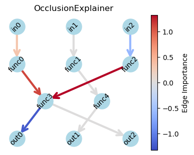
Occlusion Explainer
[20]:
tidx = 0
x = x_train[[0]]
y = y_train[[0]][:,tidx].item()
yhat = model(x.cuda())[:,tidx].item()
print('y[tidx]->', y)
print('yhat[tidx]->', yhat)

explainer = OcclusionExplainer(model, data, batch_size=64)
res = explainer.explain(x, target_idx=tidx)

plot_edge_importance(res, pos, title='OcclusionExplainer')
y[tidx]-> -1.6586637496948242
yhat[tidx]-> -1.2392131090164185
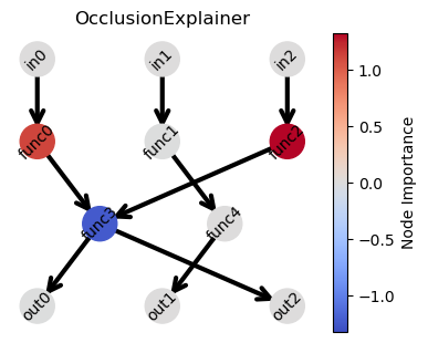
[21]:
explainer = OcclusionExplainer(model, data, batch_size=64)
res = explainer.explain(x, target_idx=tidx, target='node')

plot_node_importance(res, G, pos, title='OcclusionExplainer')
Occlusion Explainer tractability can be improved by combining with GSNNExplainer
For very large graphs, with many edges, occlusion explainer can become intractable. To improve upon this, GSNNExplainer can be used to identify a minimal subset of edges that are improtant to performance, and then these edges can be passed to OcclusionExplainer to reduce the number of edges to evaluate.
[73]:
ge = GSNNExplainer(model, data, ignore_cuda=False, gumbel_softmax=True, hard=False, tau0=10, min_tau=0.5,
                            prior=2, iters=500, lr=1e-2, weight_decay=0, beta=1, verbose=True,
                            optimizer=torch.optim.Adam, free_edges=0)

_, ge_edge_weights = ge.explain(x_train, targets=[tidx], return_weights=True)

res = explainer.explain(x, target_idx=tidx, edge_mask=(ge_edge_weights > 0.5))

res.sort_values('score', ascending=False)
iter: 499 | loss: 3.7269 | mse: 0.7279 | r2: 0.660 | active edges: 3 / 9 | entropy: 0.06496
==================================================
POST-TRAINING EVALUATION (edges > 0.5)
==================================================
Selected edges: 3 / 9 (33.3%)
MSE (subset): 0.728245
R² (subset): 0.6595
Variance explained: 0.8027
Correlation: 0.8959
==================================================
[73]:
| source | target | score | |
|---|---|---|---|
| 0 | func0 | func3 | 1.579569 |
| 3 | in0 | func0 | 0.788018 |
| 6 | func3 | out0 | -1.004601 |
| 1 | func1 | func4 | NaN |
| 2 | func2 | func3 | NaN |
| 4 | in1 | func1 | NaN |
| 5 | in2 | func2 | NaN |
| 7 | func3 | out2 | NaN |
| 8 | func4 | out1 | NaN |
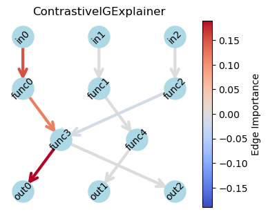
Contrastive explanations between two observations
“What latent edge features are responsible for the difference between two observations predicted outcome?”
For this example, we focus on output out0 and fix in2 to 5 for both observations, suggesting that the difference in outcome should be explained by the path from in0->func0->func3->out0.
[74]:
target = 0

x1 = torch.tensor([[0, 0, 3]], dtype=torch.float32)
x2 = torch.tensor([[-3, 0, 3]], dtype=torch.float32)

yhat1 = model(x1.cuda())[:, target]
yhat2 = model(x2.cuda())[:, target]
delta = yhat1 - yhat2

print('yhat1', yhat1.item())
print('yhat2', yhat2.item())
print('delta', delta.item())
yhat1 -5.033181190490723
yhat2 -12.176862716674805
delta 7.143681526184082
[75]:
explainer = ContrastiveIGExplainer(model, data, n_steps=100)

res = explainer.explain(x1, x2, target_idx=target)

plot_edge_importance(res, pos, title='ContrastiveIGExplainer')
res.sort_values('score', ascending=False)
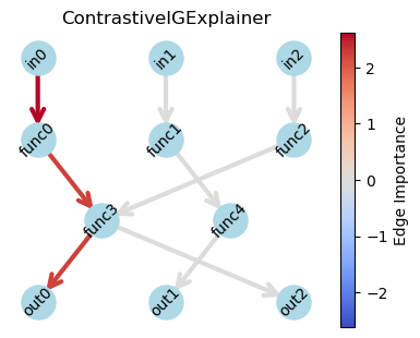
[75]:
| source | target | score | |
|---|---|---|---|
| 3 | in0 | func0 | 2.615760 |
| 0 | func0 | func3 | 2.240277 |
| 6 | func3 | out0 | 2.236099 |
| 5 | in2 | func2 | 0.034480 |
| 2 | func2 | func3 | 0.017438 |
| 4 | in1 | func1 | 0.000000 |
| 1 | func1 | func4 | 0.000000 |
| 7 | func3 | out2 | 0.000000 |
| 8 | func4 | out1 | 0.000000 |
Contrastive Occlusion Explainer
[76]:
explainer = ContrastiveOcclusionExplainer(model, data)

res = explainer.explain(x1, x2, target_idx=target)

plot_edge_importance(res, pos, title='ContrastiveOcclusionExplainer')
res.sort_values('score', ascending=False)
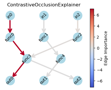
[76]:
| source | target | score | |
|---|---|---|---|
| 0 | func0 | func3 | 7.143682e+00 |
| 6 | func3 | out0 | 7.143682e+00 |
| 3 | in0 | func0 | 7.143681e+00 |
| 5 | in2 | func2 | 3.272810e-01 |
| 2 | func2 | func3 | 1.259036e-01 |
| 7 | func3 | out2 | 4.768372e-07 |
| 4 | in1 | func1 | 0.000000e+00 |
| 8 | func4 | out1 | 0.000000e+00 |
| 1 | func1 | func4 | -4.768372e-07 |
Counterfactual explanations
The goal of this approach will be to understand what minimal changes to inputs (x) can be made to change the predicted outcome to a desired value. This can be used in tandem with contrastive explainers to understand the latent changes involved in the counterfactual response.
[77]:
x = x_train[[0]]
y = y_train[[0]]
yhat = model(x.cuda())
target_ixs = [0]

# summary statistics
print('y[tidx]->', y[:,target_ixs])
print('yhat[tidx]->', yhat[:,target_ixs])
print('x ->', x)
print()

explainer = CounterfactualExplainer(model, data)

res = explainer.explain(x,
                        target_value=0.5,
                        target_idx=target_ixs,
                        dropout=0.1,
                        weight_decay=1)

print()
res
y[tidx]-> tensor([[-1.6587]], device='cuda:0')
yhat[tidx]-> tensor([[-1.0046]], device='cuda:0', grad_fn=<IndexBackward0>)
x -> tensor([[1.7641, 0.4002, 0.9787]], device='cuda:0')

Iteration 492: Loss = 0.870315
Converged at iteration 492
Final loss: 0.870315
[77]:
| feature | original | perturbation | counterfactual | |
|---|---|---|---|---|
| 0 | in0 | 1.764052 | -0.625269 | 1.138783 |
| 1 | in1 | 0.400157 | 0.000000 | 0.400157 |
| 2 | in2 | 0.978738 | -0.508059 | 0.470679 |
[78]:
xc = torch.tensor(res.counterfactual.values).view(1, -1)
cyhat = model(xc.cuda())

print('original yhat [tidx] ->', yhat[:,target_ixs].item())
print('counteractual yhat [tidx] ->', cyhat[:,target_ixs].item())
original yhat [tidx] -> -1.0046004056930542
counteractual yhat [tidx] -> -0.47705984115600586
[79]:
# combine this with a contrastive explainer

x1 = x
x2 = xc

cexplainer = ContrastiveOcclusionExplainer(model, data)

res = cexplainer.explain(x1, x2, target_idx=target_ixs)

plot_edge_importance(res, pos, title='CounterfactualExplainer')
res.sort_values('score', ascending=False)
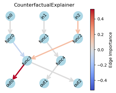
[79]:
| source | target | score | |
|---|---|---|---|
| 6 | func3 | out0 | 5.275407e-01 |
| 2 | func2 | func3 | 1.534742e-01 |
| 5 | in2 | func2 | 1.522183e-01 |
| 3 | in0 | func0 | 5.335212e-03 |
| 1 | func1 | func4 | 2.384186e-07 |
| 7 | func3 | out2 | 0.000000e+00 |
| 4 | in1 | func1 | 0.000000e+00 |
| 8 | func4 | out1 | -1.192093e-07 |
| 0 | func0 | func3 | -8.544934e-02 |
[80]:
explainer = NoiseTunnel(ContrastiveIGExplainer(model, data), n_samples=100, noise_std=0.1, agg='mean')

res = explainer.explain(x1, x2, target_idx=target_ixs)

plot_edge_importance(res, pos, title='ContrastiveIGExplainer')
res.sort_values('score', ascending=False)
[80]:
| source | target | score | |
|---|---|---|---|
| 6 | func3 | out0 | 0.189277 |
| 3 | in0 | func0 | 0.151453 |
| 0 | func0 | func3 | 0.117998 |
| 5 | in2 | func2 | 0.001137 |
| 1 | func1 | func4 | 0.000000 |
| 7 | func3 | out2 | 0.000000 |
| 4 | in1 | func1 | 0.000000 |
| 8 | func4 | out1 | 0.000000 |
| 2 | func2 | func3 | -0.013973 |
[ ]:
[ ]:
[ ]: