[1]:
from hnet.models.HyperNet import HyperNet
from hnet.train.hnet import EnergyDistanceLoss
from gsnn.models.GSNN import GSNN
from gsnn.models.NN import NN

import networkx as nx
from matplotlib import pyplot as plt
import torch
import copy
import numpy as np

from gsnn.simulate.nx2pyg import nx2pyg
from gsnn.simulate.datasets import simulate_3_in_3_out
from gsnn.models.utils import corr_score

torch.manual_seed(0)
np.random.seed(0)

%load_ext autoreload
%autoreload 2

# Bug: UserWarning: There is a performance drop because we have not yet implemented the batching rule for aten::scatter_add_
import warnings
warnings.filterwarnings(
    "ignore",
    category=UserWarning,
    module=r"torch_geometric\.utils\._scatter"
)
/home/teddy/miniconda3/envs/gsnn-lib/lib/python3.12/site-packages/torch_geometric/typing.py:124: UserWarning: An issue occurred while importing 'torch-sparse'. Disabling its usage. Stacktrace: /home/teddy/miniconda3/envs/gsnn-lib/lib/python3.12/site-packages/torch_sparse/_version_cuda.so: undefined symbol: _ZN5torch3jit17parseSchemaOrNameERKSs
  warnings.warn(f"An issue occurred while importing 'torch-sparse'. "
Uncertainty quantification with hypernetworks
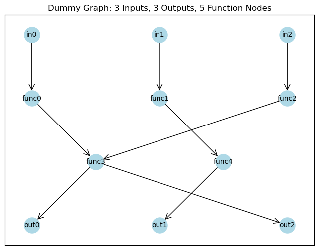
[2]:
G, pos, x_train, x_test, y_train, y_test, \
    input_nodes, function_nodes, output_nodes = simulate_3_in_3_out(n_train=25,
                                                                    n_test=250,
                                                                    noise_scale=1.)

plt.figure(figsize=(8, 6))
nx.draw_networkx(G, pos, with_labels=True, node_color='lightblue', node_size=500, font_size=10, arrowstyle='->', arrowsize=20)
plt.title("Dummy Graph: 3 Inputs, 3 Outputs, 5 Function Nodes")
plt.show()
[3]:
device = 'cuda' if torch.cuda.is_available() else 'cpu'

data = nx2pyg(G, input_nodes, function_nodes, output_nodes)
First, we’ll use GSNN wrapped in a hypernet
[4]:
gsnn = GSNN(data.edge_index_dict,
             data.node_names_dict,
             channels=10,
             layers=3,
             share_layers=False,
             bias=True,
             residual=True,
             add_function_self_edges=True,
             norm='none', # NOTE: our hypernet implementation is not compatible with batch norm
             dropout=0).to(device)

model = HyperNet(gsnn, stochastic_channels=5, width=100).to(device)

print('n params (gsnn)', sum([p.numel() for p in gsnn.parameters()]))
print('n params (hypernet)', sum([p.numel() for p in model.parameters()]))

optim = torch.optim.Adam(model.parameters(), lr=1e-3, weight_decay=0)
crit = EnergyDistanceLoss()

samples = 100
n params (gsnn) 852
n params (hypernet) 86576
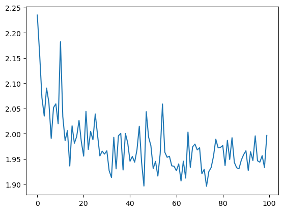
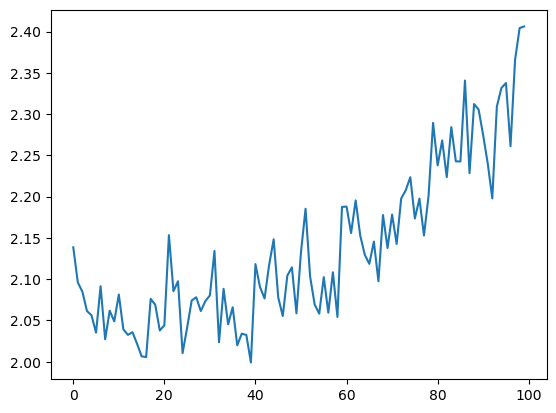
[5]:
losses_gsnn = []
for i in range(100):
    model.train()
    optim.zero_grad()

    yhat = model(x_train.to(device), samples=samples)

    loss = crit(yhat, y_train.to(device))
    loss.backward()
    optim.step()

    with torch.no_grad():
        model.eval()
        yhat_test = model(x_test.to(device), samples=samples)
        test_loss = crit(yhat_test, y_test.to(device))
        losses_gsnn.append(test_loss.item())
        r2 = corr_score(y_test.detach().cpu().numpy(), yhat_test.mean(dim=0).detach().cpu().numpy(), method='r2', multioutput='uniform_weighted')

    print(f'iter: {i} | loss: {loss.item():.3f} | test loss: {test_loss.item():.3f} | test r2: {r2:.3f}',end='\r')

plt.plot(losses_gsnn)
plt.show()
iter: 99 | loss: 1.841 | test loss: 1.997 | test r2: 0.154
[6]:
model.eval()
with torch.no_grad():
    yhat_test = model(x_test.to(device), samples=250).detach().cpu().numpy()

mse = np.mean((yhat_test.mean(0) - y_test.detach().cpu().numpy())**2)
r2 = corr_score(y_test.detach().cpu().numpy(), yhat_test.mean(0), method='r2', multioutput='uniform_weighted')

print('GSNN + HyperNet:')
print(f'\t mse: {mse:.3f}')
print(f'\t r2: {r2:.3f}')
GSNN + HyperNet:
         mse: 0.745
         r2: 0.216
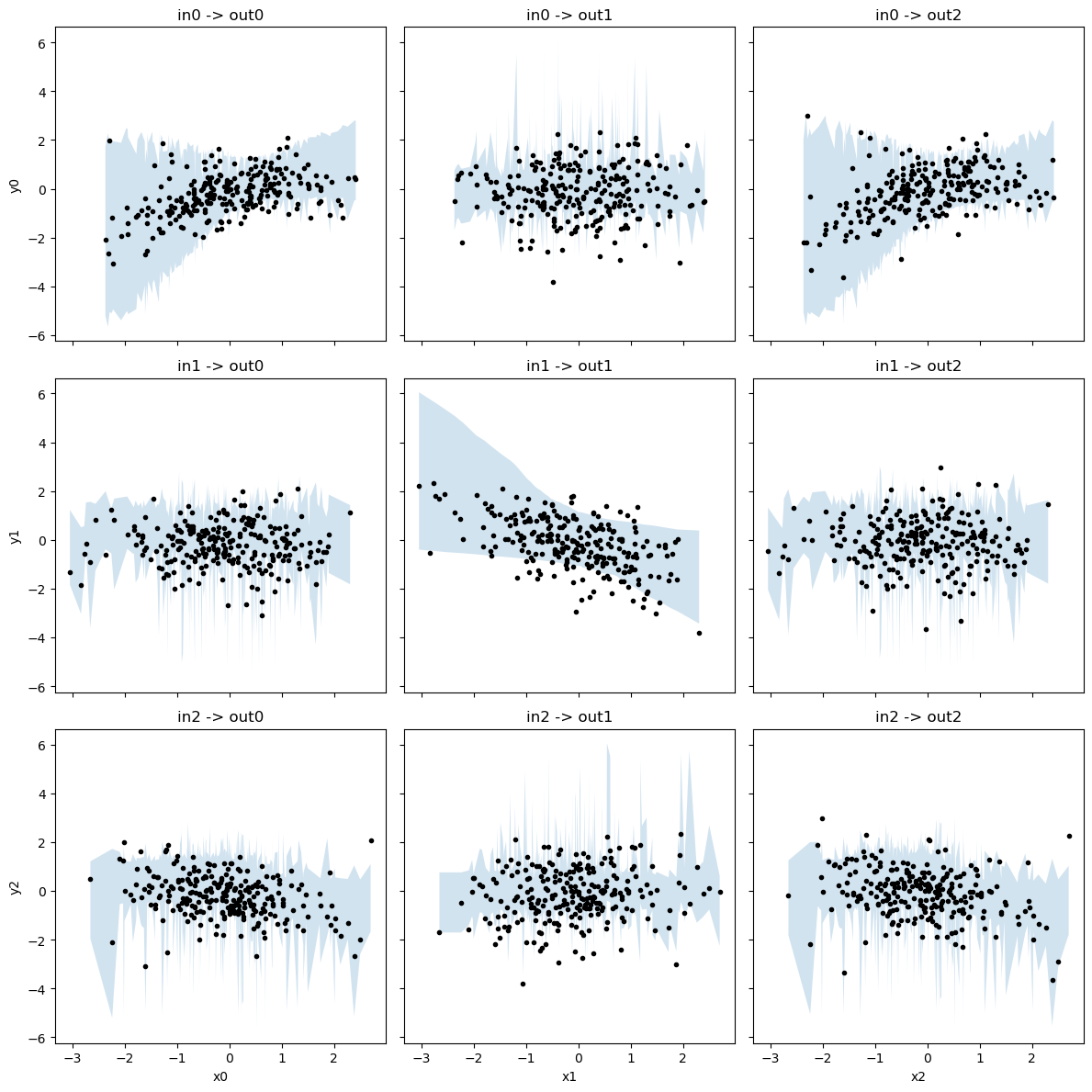
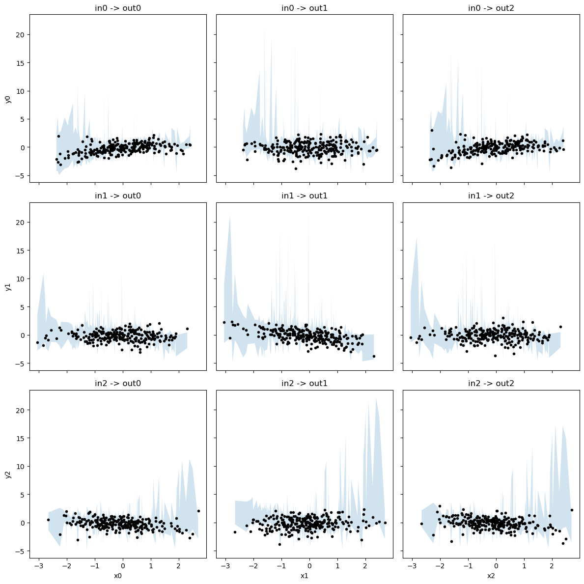
[7]:
yhat_lcb = np.quantile(yhat_test, 0.05, axis=0)
yhat_ucb = np.quantile(yhat_test, 0.95, axis=0)
yhat_mean = yhat_test.mean(axis=0)

f,axes = plt.subplots(3,3, figsize=(12,12), sharex=True, sharey=True)

for xi in range(3):
    for yi in range(3):

        axes[xi,yi].plot(x_test[:,xi], y_test[:,yi], 'k.')

        x_argsort = np.argsort(x_test[:,xi])
        axes[xi,yi].fill_between(x_test[x_argsort,xi], yhat_lcb[x_argsort,yi], yhat_ucb[x_argsort,yi], alpha=0.2)
        axes[xi,yi].set_title(f'{input_nodes[xi]} -> {output_nodes[yi]}')

axes[0,0].set_ylabel('y0')
axes[1,0].set_ylabel('y1')
axes[2,0].set_ylabel('y2')

axes[2,0].set_xlabel('x0')
axes[2,1].set_xlabel('x1')
axes[2,2].set_xlabel('x2')
plt.tight_layout()
plt.show()
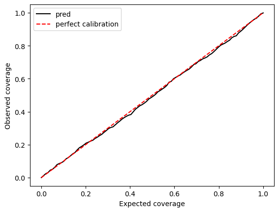
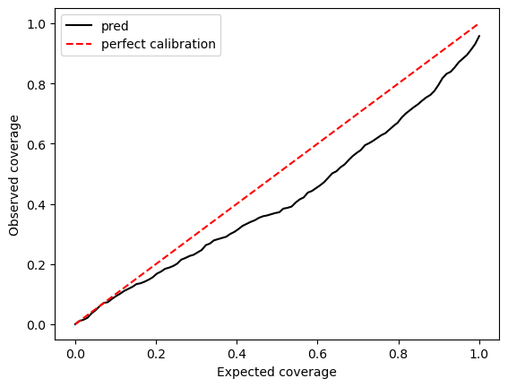
[8]:
# calibration plot

q_true = np.linspace(0,1,100)
q_pred = []

for q in q_true:
    q_lcb, q_ucb = np.quantile(yhat_test, [0.5 - q/2, 0.5 + q/2], axis=0)
    p_inside = np.mean((y_test.detach().cpu().numpy() >= q_lcb) & (y_test.detach().cpu().numpy() <= q_ucb))
    q_pred.append(p_inside)

plt.figure()
plt.plot(q_true, q_pred, 'k-', label='pred')
plt.plot(q_true, q_true, 'r--', label='perfect calibration')
plt.xlabel('Expected coverage')
plt.ylabel('Observed coverage')
plt.legend()
plt.show()
Next, we’ll compare to NN wrapped in Hypernet
[24]:
nn = NN(in_channels=3, hidden_channels=25, out_channels=3, layers=2, norm=torch.nn.Identity)
model = HyperNet(nn, stochastic_channels=5, width=100).to(device)

print('n params (nn)', sum([p.numel() for p in nn.parameters()]))
print('n params (hypernet)', sum([p.numel() for p in model.parameters()]))

optim = torch.optim.Adam(model.parameters(), lr=1e-3, weight_decay=0)
crit = EnergyDistanceLoss()

samples = 100
n params (nn) 828
n params (hypernet) 84140
[25]:
losses_gsnn = []
for i in range(100):
    model.train()
    optim.zero_grad()

    yhat = model(x_train.to(device), samples=samples)

    loss = crit(yhat, y_train.to(device))
    loss.backward()
    optim.step()

    with torch.no_grad():
        model.eval()
        yhat_test = model(x_test.to(device), samples=samples)
        test_loss = crit(yhat_test, y_test.to(device))
        losses_gsnn.append(test_loss.item())
        r2 = corr_score(y_test.detach().cpu().numpy(), yhat_test.mean(dim=0).detach().cpu().numpy(), method='r2', multioutput='uniform_weighted')

    print(f'iter: {i} | loss: {loss.item():.3f} | test loss: {test_loss.item():.3f} | test r2: {r2:.3f}',end='\r')

plt.plot(losses_gsnn)
plt.show()
iter: 99 | loss: 1.371 | test loss: 2.406 | test r2: -0.939
[26]:
model.eval()
with torch.no_grad():
    yhat_test = model(x_test.to(device), samples=250).detach().cpu().numpy()

mse = np.mean((yhat_test.mean(0) - y_test.detach().cpu().numpy())**2)
r2 = corr_score(y_test.detach().cpu().numpy(), yhat_test.mean(0), method='r2', multioutput='uniform_weighted')

print('NN + HyperNet:')
print(f'\t mse: {mse:.3f}')
print(f'\t r2: {r2:.3f}')
NN + HyperNet:
         mse: 1.713
         r2: -0.806
[27]:
yhat_lcb = np.quantile(yhat_test, 0.05, axis=0)
yhat_ucb = np.quantile(yhat_test, 0.95, axis=0)
yhat_mean = yhat_test.mean(axis=0)

f,axes = plt.subplots(3,3, figsize=(12,12), sharex=True, sharey=True)

for xi in range(3):
    for yi in range(3):

        axes[xi,yi].plot(x_test[:,xi], y_test[:,yi], 'k.')

        x_argsort = np.argsort(x_test[:,xi])
        axes[xi,yi].fill_between(x_test[x_argsort,xi], yhat_lcb[x_argsort,yi], yhat_ucb[x_argsort,yi], alpha=0.2)
        axes[xi,yi].set_title(f'{input_nodes[xi]} -> {output_nodes[yi]}')

axes[0,0].set_ylabel('y0')
axes[1,0].set_ylabel('y1')
axes[2,0].set_ylabel('y2')

axes[2,0].set_xlabel('x0')
axes[2,1].set_xlabel('x1')
axes[2,2].set_xlabel('x2')
plt.tight_layout()
plt.show()
[28]:
# calibration plot

q_true = np.linspace(0,1,100)
q_pred = []

for q in q_true:
    q_lcb, q_ucb = np.quantile(yhat_test, [0.5 - q/2, 0.5 + q/2], axis=0)
    p_inside = np.mean((y_test.detach().cpu().numpy() >= q_lcb) & (y_test.detach().cpu().numpy() <= q_ucb))
    q_pred.append(p_inside)

plt.figure()
plt.plot(q_true, q_pred, 'k-', label='pred')
plt.plot(q_true, q_true, 'r--', label='perfect calibration')
plt.xlabel('Expected coverage')
plt.ylabel('Observed coverage')
plt.legend()
plt.show()
[ ]: