Methods

Graph Structured Neural Network (GSNN)

Graph Structured Neural Networks (GSNN) were originally designed to model biological signaling networks by constraining a neural network with the structure described by a user-defined graph \(\mathcal{G}\). The graph encodes the molecular entities (nodes) and their interactions (edges), thereby defining which variables may directly influence each other during learning. The GSNN architecture is best conceptualized as univariate edge features that are transformed over sequential layer operations. The transformations are constrained by the user-defined graph, and the function nodes learn relationships between input and output edges. This approach effectively handles cyclic graphs and can scale to deep networks able to propagate information long distances through the graph.

The architecture employs three types of nodes:

• Input nodes – observed variables

• Function nodes – latent variables parameterized by neural networks

• Output nodes – target variables

Only function nodes are trainable; input and output nodes pass and receive information through the network unchanged.

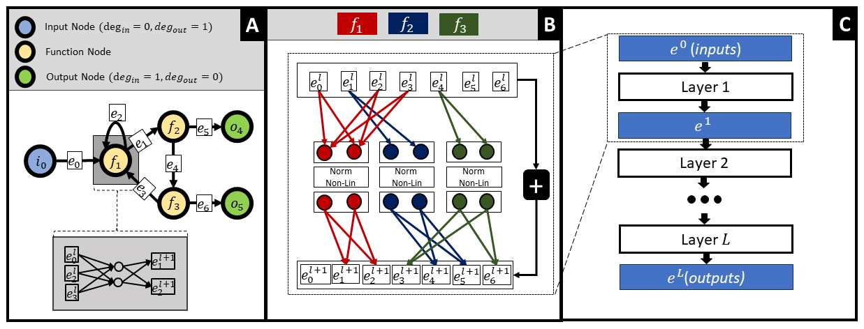
A toy example demonstrating how any given graph structure can be formulated as a feed-forward neural network with sparse weight matrices. Each yellow node in the left graph represents a fully connected one-layer neural network with two hidden channels (function nodes). Panel A shows the structural graph (\(\mathcal{G}\)) that constrains the GSNN model, while Panel B depicts how edge latent values (\(e_i\)) are updated in a single forward pass. Sparse weight matrices omit nonexistent edges, and the ⊕ symbol indicates a residual connection from the previous layer.

Note

Unlike GNNs, where latent representations typically characterize the state of a node, GSNN latent representations characterize the state of an edge. This allows the GSNN method to learn nonlinear multivariate relationships between input edges and output edges while still being applicable to cyclic graphs.

Function Nodes

Each function node \(f_n\) is implemented as a small fully-connected feed-forward network whose shape is determined by the local topology of \(\mathcal{G}\):

• Inputs – equal to the in-degree of node n

• Outputs – equal to the out-degree of node n

• Hidden channels/layers – user-defined hyperparameters. While GSNN could theoretically use multi-layer neural networks to parameterize function nodes, we have found that single-layer networks are sufficient for most applications and currently do not support multi-layer networks.

Note

To avoid confusion, we use the term layer to refer to the number of sequential sparse linear layers that propagate information across the entire graph. The neural networks that parameterize function nodes are fixed to a single layer.

Layer Updates with Masked Linear Layers

A single GSNN layer updates edge representations via a sparse linear operation. The weight matrix has shape \((E, N \times C)\) where

• \(E\) – number of edges in \(\mathcal{G}\)

• \(N\) – number of function nodes

• \(C\) – hidden channels per function node

Note

There is no parameter sharing between function nodes—each learns a distinct mapping from its inputs to its outputs. That said, parameters can optionally be shared across layers.

Iterating the update L times enables information to travel a path length of L across the input graph.

Sparse Implementation

A dense implementation of the masked matrices would quickly exhaust memory on realistic graphs. Instead, GSNN stores the matrices as sparse tensors, reducing both memory and compute. The current PyTorch sparse backend is not optimized for mini-batching, so GSNN leverages PyTorch Geometric for fast batched sparse matrix multiplication, especially on GPUs.

Residual Connections & Normalization

GSNN is [optionally] a residual architecture where the layer output is added to its input:

\[x_{l+1} = F(x_l) + x_l\]

Residual connections allow the model to learn edge latency—the temporal lag between upstream and downstream signals—and alleviate vanishing gradients in deep networks.

• Normalization – We provide several normalization options:

  • layer – Group layer normalization applied within each function node. Works well for small batches with large channel sizes.

  • batch – Standard batch normalization applied within each node channel. Works well for large batches and small channel sizes.

  • groupbatch – Group-wise batch normalization that normalizes within channel groups.

  • edgebatch – Edge-level batch normalization applied before the sparse linear operations.

  • softmax – Softmax normalization applied within function nodes (activations sum to 1 per node).

  • rms – Root Mean Square normalization, simpler and more stable than layer norm for small batches.

  • ema – Exponential Moving Average normalization for more stable training.

  • channelema – Channel-wise EMA normalization.

  • none – No normalization is applied.

• Self-edges – Optional addition of self-edges in the structural graph, which allows dependence on the previous layer state.

• Parameter sharing – While GSNN supports weight sharing across layers, empirical results typically show better performance when each layer has its own parameters.

• Node MLPs – Optional additional MLP processing per node to enhance representational capacity while maintaining graph structure constraints.

• Node attention – Optional attention mechanism applied to node representations.

• Learnable residual weights – Residual connections can use learnable scaling factors.

Weight Initialization

GSNN offers comprehensive weight initialization strategies adapted to the graph setting. Let \(D_i^{in}\) and \(D_i^{out}\) be the in- and out-degree of function node i in \(\mathcal{G}\). The following initialization methods are available:

• Xavier/Glorot methods: * xavier_uniform: Uniform distribution scaled by \(\sqrt{\frac{6}{D_i^{in}+D_i^{out}}}\) * xavier_normal: Normal distribution scaled by \(\sqrt{\frac{2}{D_i^{in}+D_i^{out}}}\)

• Kaiming/He methods: * kaiming_uniform: Uniform distribution scaled by \(\sqrt{\frac{3}{D_i^{in}}}\) * kaiming_normal: Normal distribution scaled by \(\sqrt{\frac{2}{D_i^{in}}}\)

• Simple distributions: * uniform: Standard uniform distribution with configurable gain * normal: Standard normal distribution with configurable gain * zeros: Initialize all weights to zero

• Graph-aware initialization: * degree_normalized: Applies GCN-style degree normalization \(D^{-0.5}AD^{-0.5}\) to uniform weights

Using degree-aware fan-in/fan-out preserves the variance of activations despite the sparse, non-uniform connectivity. The default initialization is degree_normalized, which often performs well across different graph topologies.

Efficient Mini-batching

PyTorch’s native sparse operations remain slow for large batches. GSNN therefore reformulates the masked linear layers as PyTorch Geometric graph convolution, gaining substantial speedups during training and inference—particularly on GPUs. The implementation automatically handles batching of sparse operations and edge indices.

Gradient Checkpointing

To reduce memory usage, GSNN supports gradient checkpointing at each layer, which substantially reduces memory usage at the cost of some additional compute during the backward pass.

Advanced Features

Node MLPs GSNN supports optional Multi-Layer Perceptrons (MLPs) applied to each function node’s representation. This enhances the representational capacity while maintaining graph structure constraints. The node MLPs process channels within each node independently, allowing for more complex transformations without violating the graph structure.

Node Attention An optional attention mechanism can be applied to node representations, allowing the model to dynamically weight the importance of different nodes during computation.

Edge Weights GSNN supports weighted edges through the edge_weight_dict parameter, allowing different edge types to have learnable or fixed importance weights.

Flexible Residual Connections Residual connections can use learnable scaling factors, providing more flexibility in how skip connections contribute to the final output. The residual weight can be learned during training or kept fixed.

Multiple Edge Channels The model supports replicating edge features across multiple channels using the edge_channels parameter, enabling richer edge representations.